Stats for Spikes-Control Charts

I am sure that I am not the first, nor the last, to want to apply Statistical Process Control analysis to volleyball statistics. Here is my attempt with control charts.

I became familiar with Statistical Process Control (SPC) when I was working in engineering and having to understand the manufacturing world.

As I learned about SPC, I was eager to apply the methodology to volleyball because the philosophy behind SPC seems to be ideal for coaches to use to take their team’s pulse through their team’s statistical performances over time. The most basic and easily applicable tool from all the SPC arsenals is the control chart.

What foolow is a short historical synopsis of SPC, this is my appended history and description of SPC of what is in Wikipedia, any mistake is all mine. (https://en.wikipedia.org/wiki/Statistical_process_control)

Statistical Process Control (SPC) or Statistical Quality Control (SQC) is the application of statistical methods to monitor and control the quality of a production process. This helps to ensure that the process operates efficiently, producing more specification-conforming products with less waste scrap. The process can be a single component or a series of interconnected components. The SPC was the brainchild of Walter A. Shewhart at Bell Laboratories in the early 1920s. Shewhart developed the control chart in 1924 and the concept of a state of statistical control.

W. Edwards Deming invited Shewhart to speak at the Graduate School of the U.S. Department of Agriculture and served as the editor of Shewhart's book Statistical Method from the Viewpoint of Quality Control (1939), which was the result of that lecture. Deming was the architect of the quality control short courses that trained American industry in the new techniques during WWII, but the lessons were ignored by American industry because American industry was booming post war, and the management did not worry about quality, just volume.

The US government introduced and helped educate post-World War II Japanese industry by sending Deming to Japan during the Allied Occupation. He met with the Union of Japanese Scientists and Engineers (JUSE) to introduce SPC methods to Japanese industry, and to assist the Japanese economy to recover from the devastation of the War.

The Japanese manufacturers integrated SPC into their manufacturing process and implemented quality improvements on their manufacturing.

Ironically, the Japanese industry introduced SPC methods back to American industry when the Japanese manufacturing excellence gained renown globally. The SPC idea also evolved and spawned several other quality improvement methods based on the SPC ideas that became ubiquitous in the manufacturing world: Six Sigma, Total Quality Control (TQC), et. al.

There are several assumptions associated with SPC that have been integrated into the way we think about complex systems, i.e., systems that are composed of many components, with each component functionally related to other components of the system.

· A process/system is more than the sum of the parts; the process consists of numerous components. The process is a system.

· The process/system can also be a sub-system of a larger and more complex system.

· The components making up the system are interconnected and interdependent, i.e., the system acts in a nonlinear manner.

· Many times, the process/system is treated as a black box because the process/system cannot be understood or modelled by just measuring the input and output of the process/system, i.e., the relationship between input and output is not scalable, or linear.

· Intermediate variables can also serve to change the trajectory of the process, i.e., these control variables can affect system performance, if we can get access to them.

But.

· Not all variables are measurable; these unmeasurable variables could possibly be critical to monitoring and understanding the process/system flow.

· Not all variables are control variables.

· Not all variables are controllable.

The abstract idea of a complex system sounds suspiciously like a sports team playing the game.

A “system” is an abstraction that is applied to the process that is being measured and monitored. In the case of volleyball statistics, the “system” can be defined as a player, or it can be defined as all the players participating in team play. This is important because of the nature of sports statistics; they can be objective termination statistics — point scoring statistics — or subjective evaluation statistics — ranking of the pass, as an example. Since the action in sports do not reside only in those statistics that we can measure, the statistics that we measure do not factor in all the impact of the intermediate actions, which also introduces variability to the system performance that cannot be accounted for objectively within the statistics that we can measure; this is problematic when coaches are trying to evaluate their players — individually or together.

There are other sources of variability, the resistance that the opponent presents to the team under assessment is also highly variable; as such, the performance statistics will also be highly variable and dependent on the opponent. Other sources of variability are: the emotional and physical states of the teams at a specific point in time for both the team that is being assessed and the opposing team, the playing environment, the officiating thresholds that is applied during the contest, the emotional and physical states of the officials at a specific point in time, the consistency of the data taking process, et. al.

All that variability is built into the statistical measurement practices, and since the practice of keeping statistics is performed in terms of averages, the salient sources of variability are smoothed out. Additionally, the rules governing the interpretation of the control chart will also take those sources of variability into account.

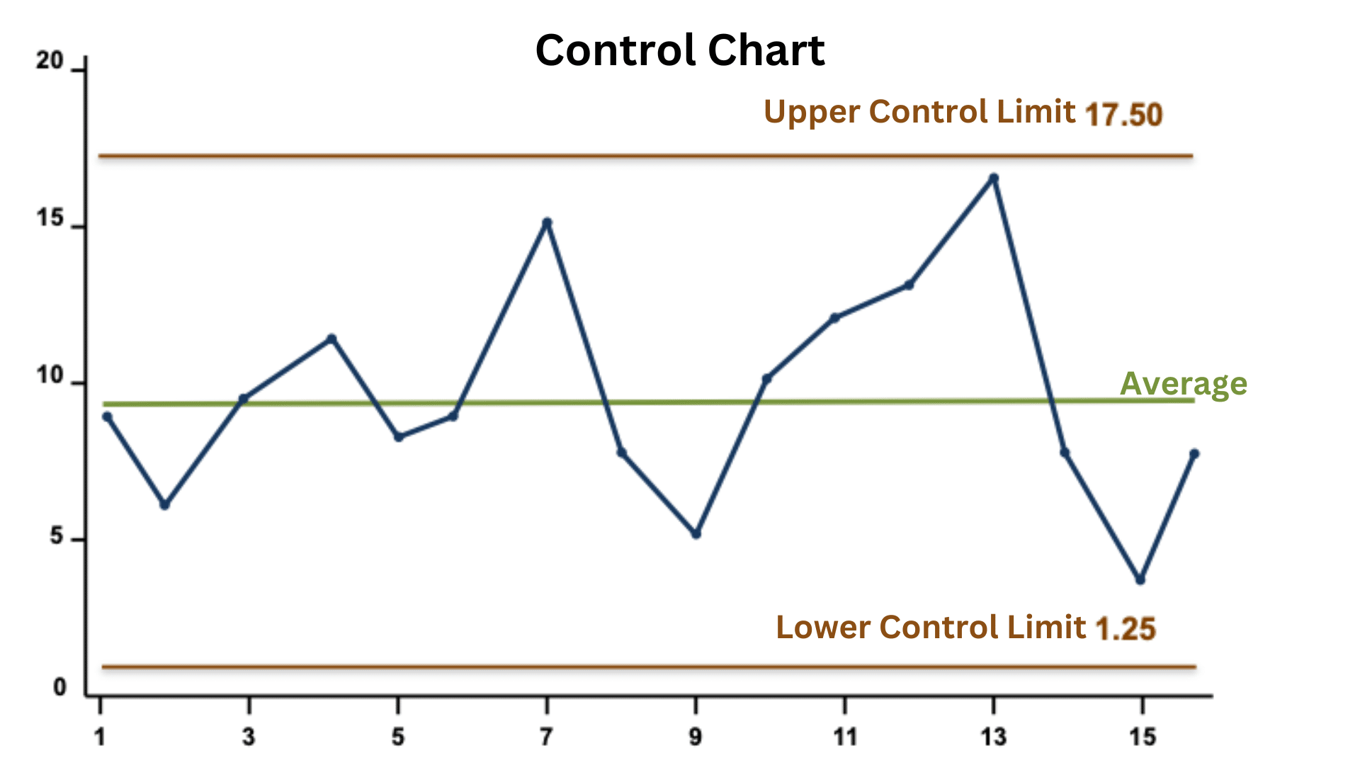
A control chart is the simplest, most ubiquitous, and — in my mind at least — the most promising SPC tool that can be applied to volleyball statistics. This is because the control chart does not involve specialized statistics that is unfamiliar or unintuitive to coaches; it is instead a way to look at the accrued statistics already taken by the coaches as a matter of assessing the team performance over time (see Figure 1). The control chart analysis gives the coaching staff a chance to examine team performance over a time period (the pre-season, the conference season, etc.) to assess and identify trends in the team’s performance. The performance statistics are presented visually so that the coaches are not otherwise overwhelmed with processing the data in their working memory. Coaches already examine these statistics over time, but presenting the data visually is much simpler to comprehend and gives the coaches a chance to interpret the data from a broader perspective.

The dashes on the horizontal axis represent each event for which a data point is available, a chronological progression is assumed as the numbers are incremented from left to right. In the case of volleyball, each event represents a match or even a set, although using set data can lead to confusion when analyzing the control chart, as they will show up in the interpretation of the special cause rules.

The vertical axis is the statistic associated with each event. The average is the arithmetic mean (or simply mean or average) of a list of numbers, is the sum of all the numbers divided by their count n.

To calculate the upper control limit (UCL) and lower control limit (LCL), the mean is augmented by the standard deviation of the entire series. The standard deviation is the square root of the variance of the data series, and the variance is defined simply as

Figure 1: A Control chart. https://deming.org/wp-content/uploads/2023/06/Control-Chart-v2.png

In manufacturing, the control chart is used to monitor the performance of machines and processes. Statistics are taken of many variables that monitor the production of a process, whether they consist of a single or in a complex system made up of many machines.

If we want to use the same method to monitor a sports team, there is a tacitly accepted assumption that a team, made up of many autonomous human beings, can be treated as a system. One salient problem with using the control chart to examine the performance statistics is that human actions and reactions are more variable than machines, the behavior of the measured performances over time are also more variable in the control chart analysis. This variability is also visible in the control chart, which indicate that team performances are more susceptible to wider variations; but some of the wider variations have meaning while others are just a function of natural human behavior, it gives the coaches analyzing the control chart more leeway in interpreting the trends, as will be seen when discussing the common and special cause rules. This human proclivity to be more variable needs to be kept in mind even though the analysis tool for the control chart, by its nature, can account for some of those variabilities.

Any set of volleyball statistics can be plotted as a control chart.

Every termination statistic can be examined with the control chart. (https://thecuriouspolymath.substack.com/p/stats-for-spikes-termination-scoring?utm_source=publication-search): attacking, serving, reception, blocking, digs etc.

Sometime coaches assign quality grades to the intermediate actions, such statistics as service quality, first touch quality, set quality, etc. They are fair games as well, except that the quality grades assessment must be consistent to avoid introducing more variability because of the subjectivity in grading.

There are two main groupings of the variations that are represented in the control chart: common cause and special cause. The explanation of the difference between the two can be found in the following reference. https://www.isixsigma.com/control-charts/common-cause-vs-special-cause-variation-whats-the-difference/

It is important to understand the differences between these two variations because the differences determine whether and how issues need to be adjusted with the process/system.

Common cause variation is the kind of variation that is part of a stable process. These are variations that are natural to a process/system, are quantifiable, and expected; they are predictable, ongoing, and consistent. Major changes rather than cursory adjustments must be made to change the process/system trajectory because the process/system has settled into a steady state behavior or rhythm.

In the volleyball context, the statistics measure, whether it is passing grades, or termination stats like kill percentage will vary in between the control limits, UCL and LCL. The variations seen in the statistical behavior variation with time account for the variation in the opponent resistance, the mental and physical states of the teams competing, the playing environment, the officiating thresholds that are applied, and the consistency of the data taking process.

Since common cause variations are always present, they are measured to establish a baseline for comparison. These types of variations also fit easily within the control limits of a control chart. The identifying characteristic of common cause variation on the control chart is its random pattern of variation and its adherence to the control limits. The system is termed as being in control when all the variations that appear are common cause points.

An in-control system tells the coach that their team is performing without excessive variations, the team’s performance has settled into a steady state, and the team is acting and reacting predictably to predictable challenges during competition; that is, the resistance from opponents and circumstances are within the team’s capabilities.

The downside of being in-control is that if the in-control system performance metric does not meet the expectations necessary to compete against familiar opponents: if the coaches have a predetermined threshold for the performance metric, that performance metric cannot be improved without imposing major changes to the system. For example, if the control chart is applied to first touch quality point, where a pass is rated a 3 for a pass that allows the setter to set to all hitters, a 2 for a pass that allows the setter to only set the pin hitters, a 1 for a pass that allows the setter to only set the backrow hitter or if the hitter can only freeball or down ball to the opponent, and a 0 for a pass that is an error. The heuristic that is usually applied is to correlate an average passing quality metric of 2.4 with being successful; but, if the first touch quality point for the in-control team is 1.5, significant changes must happen to the serve receive system to improve that number; the changes can range from changing formations, changing primary passers, changing serve receive patterns, etc. The key lesson for the in-control system is that nothing will change if they just keep doing what they are doing.

https://www.spcforexcel.com/knowledge/control-chart-basics/control-chart-rules-interpretation#control-chart-review

Special cause variations are unexpected variations that significantly affect a process/system. It is also known as “assignable cause” because the special cause that manifests itself in the control chart can be assigned to specific reasons. These variations are unusual, are not readily explainable, are not previously known, nor can they be anticipated. They are the result of a specific change that has occurred in the system, which results in the process/system being out of statistical control. These specific changes can take the form of changes in the challenges posed by the opponent and changes within the process/changes. The difference is important, but the result is the same since the teams can only control what they can control and not control what they cannot control: the process/system must adapt to the changes in the resistance that the opponents present or adapt to changes that had crept into their own process/system.

Special cause variations are due to a specific defect in the process/system that MAY be identifiable and reparable. Referring to the first ball passing example, a special cause analysis can be attributed to a team’s inability to pass short serves, or deal with float serves.

Contrary to the common cause variations, special cause variations on a control chart are identifiable by their non-random patterns and out-of-control points.

There are eight specific patterns on the control chart which can be called special causes.

Zone A is defined as the zone between

and

, or between

and

.

Zone B is defined as the zone between

and

or between

and

Zone C is defined as the zone between

and

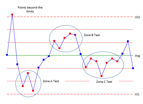
Rule 1: Beyond limits. One or more points beyond the control limits

Rule 2: Zone A. 2 out of 3 consecutive points in Zone A or beyond

Rule 3: Zone B. 4 out of 5 consecutive points in Zone B or beyond

Rule 4: Zone C. 7 or more consecutive points on one side of the average (in Zone C or beyond).

Rules 1 (points beyond the control limits) and 2 (zone A test) represent sudden, large shifts from the average. These are often fleeting – a one-time occurrence of a special cause – like if a team of ten-year-olds played the national team for Rule 1 and if that same ten-year-old team played a series of matches with the national team for Rule 2. Note that Rule 2 specifies 2 out of 3 consecutive points in Zone A, meaning the variations are close to the control limits, meaning that 2 of the 3 points recorded are triple that of the standard deviation σ of the process/system measured steady state capability.

Figure 2 Rules 1-4 for special causes. https://www.spcforexcel.com/files/images/control-charts-rules-pics/rules-1-4.png

Rules 3 (4 out of 5 consecutive points in Zone B) and 4 (7 or more consecutive points are in Zone C) represent smaller shifts that are sustained over time. The key is that the shifts are maintained over time — at least over a longer period than Rules 1 and 2, that is, having more consecutive points residing in the narrower neighborhoods of interest. Given that human actions in sports are much more variable than automated machines that the control chart is intended to monitor, Rules 3 and 4 may be ignored unless the coach has specific reasons for suspecting that these small variations are appearing. The first consideration is to examine the scale of the standard deviation, if the σ is a small percentage of the mean, this could indicate that the system is unresponsive and stagnating. The downside of that is that the process/system may not be capable of responding to extraordinary challenges from the opponent, but some coaches prefer that their process/system is more predictable and less prone to variation.

It is a part of a coach’s human nature to want the system (the team) to behave deterministically or minimize surprises. Coaches will often take action to minimize the variations — reducing the σ — deeming all variations detrimental. This is a sign that the coach grossly misunderstands statistics because randomness and variation are a part of the natural order, especially when the system consists of humans interacting in real time. Randomness and variation are not only to be expected but are necessary for a dynamic and responsive process/system, especially in sports.

Rules 1, 2: Large shifts from the average.

Rules 3, 4: Small shifts from the average.

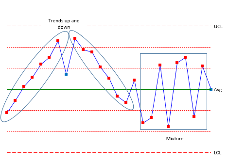
Figure 3 Rules 5 and 6.https://www.spcforexcel.com/files/images/control-charts-rules-pics/rules-5-6.png

Rule 5: Trend. 7 consecutive points trending up or trending down.

Rule 6: Mixture. 8 consecutive points with no points in Zone C.

Figure 3 shows Rules 5 and 6. Rule 5 (7 consecutive points trending up or trending down) represents a process/system that is adjusting or changing. Trends can indicate that the team/system in the process of integrating new skills or techniques while competing; players learning new things while performing in matches will always struggle, especially early in the learning process. It is important and insightful to monitor the trending to see if the trend continues beyond the seven consecutive points and whether a reversal of the trend occurs, indicating that the team/system have learned and adequately integrated the changes into their knowledge base: they have switched from thinking and learning mode to playing mode, to the exclusion of overthinking.

Rule 6 (mixture, 8 consecutive points bouncing above and below Zone C) occurs when there is more than one system present. For example, if the coach is playing different lineups but is keeping the statistics in a single control chart. This practice presumes that both lineups are performing at the same average while one lineup is operating at a different average than the other lineup. The giveaway is the alternation of the data in Zone B

without having any data in Zone C

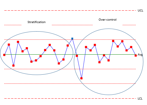
Figure 4 Rules 7 and 8. https://www.spcforexcel.com/files/images/control-charts-rules-pics/rules-7-8.png

Rule 7:nStratification. 15 consecutive points in Zone C.

Rule 8: Over-Control. 14 consecutive points alternating up and down.

Figure 4 shows rules 7 and 8. Rule 7 (stratification), which also occurs when the statistics of multiple lineups are combined, the calculated average for different lineups is grouped into one, which causes the plot to vary in this way. This can lead to the data “hugging” the average — all the points in zone C with no points beyond zone C. Rule 8 (over-control) is often due to over adjustment. This is often called “tampering” with the system/process. Adjusting a lineup or changing the way the team is playing while it is in statistical control actually increases the process/system variation, that is the price of making changes, which we are all willing to do if the intent is to improve team performance, increasing win and decreasing losses. But, if a coach is manipulating the team/process solely to meet performance metric goals, they are violating Goodhart’s Law, which I have discussed before. (https://polymathtobe.blogspot.com/2022/07/stats-for-spikes-goodharts-law-and.html) Briefly, Goodhart’s Law is: “When a measure becomes a target, it ceases to be a good measure.” It manifests itself in the saw-tooth pattern from Rule 8.

While it may seem common sense to use specific metric values as target, it focuses attention on meeting the target of a single dimension of a multidimensional task. The reason for monitoring the single dimensional metric is to assess that part of a vast complex process/system performance; by focusing on a single dimension and making it the goal is losing sight of the forest because of one tree. In mathematical terms, local optimizations (isolated view of a single part or action) are the priority over global optimization (broad view of the combined process/system).

Given the length of the volleyball season, it may be a long time before the trends begin to make itself visible. One practice to implement is to use initial practice stats or scrimmage stats to get the statistical timeline started. The problem is that practices and scrimmages are different from match play, but using these statistics is akin to priming the pump, so to speak. Coaches can choose to keep those statistics in the seasonal timeline as the season evolves, or they can choose to retire those startup statistics as they get more match statistics.

The two key statistics used for the control chart: the mean and standard deviation will also vary as the season evolves. It is useful to track their variations during the season to assess how the team performance in those statistical categories is evolving. There may be times when there are significant breakpoints in the mean and standard deviations which mark changes in the way the process/system has changed in their performance.

The control chart is a relatively simple tool to use, any spreadsheet program can be used to handle the plotting and calculation tasks, many software has built in statistical functions that will plot the control chart with UCL and LCL. It is a tool that examines team performance in specific categories as the season progresses, the insight that the control chart offers is dependent on the trends illustrated in the charts.

As with everything in life, the interpretation of the control chart rules is dependent on the interpreter. As I had stated earlier, this is a tool intended to monitor machines and automated processes, which are not as variable as humans, particularly humans that are working together as a team; it is therefore important to allow greater variations, σ, with the process/system statistics and with the interpretations of the special cause rules because it is very easy to become overly alarmed by the control chart and try to control what does not need to be adjusted. On the other hand, the control chart does illustrate the kind and amplitude of variations that exists in a process/system. It is up to the coaches by using their experiences and knowledge to decide whether they should intervene in a meaningful way. The advantage of the control chart is that it gives the coach a tool to either reinforce or refute their coaching instincts over a greater range of performances as marked by time, which gives the coach a picture of how the team is developing.

I hope this is useful.